The LITTLEMORE Clock - June 1996
By Prof E.T. Hall, Oxford, England
It has been a mystery to me for many years as to why pendulum clocks, even the most accurate so far made are not more precise over long periods. This is why I started some years ago looking into the problem and trying to improve accuracy to the ultimate and, at the same time, find out the causes of instabilities in performance.
Description of equipment
- Clock movement
The pendulum is similar to a standard seconds type (e.g. Synchronome). The rod (9.6 mm diam.) and bob (75 mm diam.) are made from 15 year old Invar. The bob weighs 6.4 Kgm.
Temperature compensation is by the use of a composite slug of Invar and Type 304 stainless steel. This 25 mm diam. slug is inserted into the base of the bob as shown in Fig. 1. The rating nut of Invar has a 20 TPI thread giving a change of rate of 1.6 S/Hr per turn. The top of the bob is engraved with 36 divisions giving a change of rate of 46 ms/Hr/division. The ratio of the lengths of Invar and stainless was found by experiment to give a minimum temperature coefficient (45.5mm Invar, 38.5mm stainless).
Figure 1 - Pendulum Bob
The support of the pendulum assembly consists of an aluminium plate (300 x 230 x 19 mm) firmly fixed to a concrete pillar by stout screws. This plate in its turn supports another plate (230 x 170 x 19 mm) via a central 16 mm diam. bolt and clamping nut. This second plate, which carries the pendulum, can be rotated and clamped by two jacking screws when the pendulum has been set so that the shutter (see below) is exactly central when the pendulum is stationary. The verticality of this plate in the front/back plane is adjusted by means of four other jacking screws.
The suspension of the pendulum is by means of a pair of inverted 60° agate prisms resting on a plane agate surface. The prisms are held in a rectangular bar of Invar, the pendulum passing through the block and between the prisms. The pendulum can swing in the front/back plane, since it is fixed to the block via two small ball races and a 3 mm shaft ,which is a push fit in the pendulum shaft (Fig. 2). A lever system, controlled by a manual screw, lifts the pendulum off the bearing plane allowing it to rest in a pair of crutches when not in use.
Figure 2 - Pendulum Suspension
Impulses to the clock are provided electromagnetically every two seconds by means of a copper wire coil mounted to one side of the pendulum. Many writers on horology have decried magnetically maintained pendulums they are unreliable, they cannot be given an absolutely constant impulse etc. However if the correct design is used, they are both very reliable and, as we will see, give exceptional results as far as accuracy is concerned. In particular two points are important:
- A constant current as opposed to voltage control must be used; this prevents changes of resistance due to temperature having an effect on the current through the coil. Modern electronics allow control of current to better than 1 ppm, if appropriate circuitry is used.
- All electrical contacts must be eliminated for both reliability and to enable the pendulum to be 'free'.
Seconds detection and phase measurement: A circular aluminium plate is mounted just below the pendulum; it is mounted on three long spacers from under the suspension plate. On the top side of this plate a LED/photodiode assembly is fixed so that a shutter attached to the bottom of the pendulum interrupts the light between the LED and diode except when a 1.6 mm wide slot in the vane allows light to pass. This signal from the diode is used for three purposes for counting the seconds, to enable the amplitude of each swing to be measured (see below) and to monitor any tilt of the suspension pillar.
A vacuum housing surrounds the pendulum: this consists of a glass tube (150 mm diam. 1100 mm long, 8 mm wall) with short aluminium end tubes glued to the glass for clamping the sections of tube: Viton 'O' rings are used as seals.
The high vacuum is provided by a turbo molecular pump (30 litres/sec) backed by a small 2 stage rotary pump (0.5 litre/sec). The latter gives a vacuum of 0.2 mbar, whilst the former a final pressure of 2 x 10⁻⁶ mb.
The clock house, measuring 1.5 meters square, is built next to an existing small timber laboratory. It is separated from the laboratory by a double glazed Perspex window. The temperature within the clock house is maintained at 32°C ± 0.05°C by means of a Pt resistance sensor controlling electric elements and fans.
Within the clock house, a mounting column has been erected. Above ground, the concrete column, to which the clock is fixed, measures 600 mm square by 2.5 meters high. This is mounted and firmly fixed by stainless reinforcing bars to an underground concrete base measuring 1.2 meters square by 3.5 meters deep weighing about 12 tons. This base is separated from the surrounding soil by a 50 mm layer of expanded polystyrene. The object of these somewhat elaborate precautions is to prevent as far as possible any vibrations from local sources. Indeed the improvement in the performance of the clock since these precautions were taken is very marked as is indicated from both amplitude variations and time keeping.
Adjustment of rate. There are four methods of making such adjustments:
- The rating nut at the bottom of the pendulum moves the bob vertically. There are 36 divisions on the top of the bob. One division movement changes the rate by ± 46 ms/Hr.
- A small horizontal tray is carried on an extension to the pendulum about 100mm above the suspension. Addition of 1 gm to this tray will slow the clock by 30 ms/Hr.
- A 40 turn single layer bias coil with its axis vertical is wound around the glass envelope at the height of the centre of the bob. Passing a current through this coil will cause a change of rate of 3.3 ms/Hr/ma. A current stabilised power supply with a 10 turn control provides this current.
- A change of pressure will alter the rate. The rate coefficient for pressure is 0.77 ms/Hr/mb. However since the clock operates at < 10-5 mb, changes in this pressure region will have negligible effects on rate. However this effect should be kept in mind when initially setting up in air.
- Associated Equipment
- Clock readout. The pulses from the LED/diode assembly within the vacuum chamber are fed to this unit via a vacuum seal. By the use of appropriate digital counters and 25 mm high LED displays, a 12 hour clock is provided. All the required logic and drive circuitry is contained within this unit. Controls are provided on the clockface for setting time and also for setting the phase of the swing of the pendulum to coincide with the clock such that the impulse is only given when the pendulum is approaching the impulse coil
- Clock comparator. This unit compares the time of day displayed on the clock with that time registered within the unit, driven by an oven stabilised 5 MHz quartz crystal, having a long term frequency stability better than 1 part /108/ year. The error is computed and displayed each minute to 0.1 ms. This reading is also registered by the recorder each minute and sent to the computer at the hour to a sensitivity of 0.1 ms (averaged over the hour).
- Use of GPS frequency standard. Though time is measured by comparison with a 5 Mhz crystal with a rate of 10-2 ppm/year, the cumulative error will be 50 mS / year. It is now easy to compare the clock with UT1 using a satelite GPS (Global Positioning System). Some apparatus provides a 20 S wide pulse at the start of every second. By using a gating system and a 10 KHz crystal we have made an instrument which provides the decimal fractions of the current second on a 5 figure LED display at 4 second intervals.
- Amplitude readout. As explained above, a shutter attached to the bottom of the pendulum swings between an LED and photodiode in such a way that light passes from the one to the other only when a 1.6 mm slot in the shutter allows it to do so. As I shall show below, the angular amplitude is directly proportional to the maximum pendulum velocity at its midpoint of swing. We can arrange that the slot is at this central point when at rest: it will also have its maximum velocity at this point when swinging. During the period that the light passes it can be arranged that an electronic gate is opened and whilst the gate is open a 1 MHz signal is allowed to pass to a counter. These counts are accumulated at each pass of the pendulum (60 times per minute). At the end of the minute the first four figures of the accumulated seven figure number are passed to the recorder and the average value of these figures is sent to the computer at the hour. This figure is inversely proportional to the amplitude. Fig. 9 illustrates this system.
Figure 9
- Computer and Printer. A PC computer is connected to the system. This has a number of functions:
- At each hour the computer program passes the values of average time and average amplitude to files both on the harddisk and on the floppy. The latter can be taken (during non recording periods) to an external computer for processing the results.
- Various parameters can be monitored and continuously recorded by being passed to the computer. Amplitude and pillar tilt are obvious examples.
- The computer is used to stabilise the amplitude. The system works as follows. At the start of a run a value of the amplitude is chosen (this will be a 4 figure value as described above). By experience a value of the impulse coil current a little above that necessary to maintain this amplitude is also chosen and set by a potentiometer on the clock readout panel. At each minute the last measured average value of amplitude is compared to the set value and if the former indicates a higher amplitude to that set, no impulse will be given for the next minute. This procedure will continue until the measured amplitude exceeds the set value. Because the clock operates in a high Q regime some -'hunting' may occur for several hours until the system stabilises.
- The printer is used to continuously monitor the time and amplitude drift on paper.
- Pressure measurement. A commercial Pirani gauge is used to monitor the backing pump pressure. The clock case pressure is measured by a cold cathode ionisation gauge which uses a strong permanent magnet. It has been thought wise to remove this magnet as far away as convenient so as to obviate changes of clock rate due to drifts of the associated magnetic field. In fact it is mounted on a 500 mm long 50 mm diam. aluminium tube. Whilst on this subject, it is worth mentioning the importance of removing any potentially disturbing magnetic objects or fields; this particularly concerns those which might get moved after setting up the equipment, e.g. metal chairs or pieces of apparatus.
- Standby power and alarm. It is most important that long runs of results should be protected and that continuity should be preserved. Since all results are recorded every hour in two places protection is secure. It is important that the following devices do not stop on a mains failure; backing pump, turbo pump, computer, amplitude monitor (which also provides power to the clock and impulse system) and rate adjustment bias coil supply. All these units are mains powered from inverters, which convert 24 volts DC to 230 2 volts AC . The 24V DC is provided by two 12V car batteries in series; they have a capacity of 150 AH. The batteries are kept charged by AC operated power supplies with a capacity of 25 amps. If the mains fail, the battery/inverter system will maintain accurate time for at least 4 hours. At the same time an alarm will sound, which will signal 'panic stations'; it is hoped that this time interval will allow emergency steps to be taken. A standby 1.5 kW petrol driven generator is on site and, by means of a simple changeover switch, can take over from the mains until repairs are effected.
- Pendulum tilt detector. As has been stated above, the whole clock assembly is firmly fixed to a cast concrete pillar. Although it is hoped that this pillar is completely stable, we cannot be sure that it is so and how can we verify this? When setting up the clock, we adjusted the left/right jacks to allow the pendulum to swing centrally by eye. We have now incorporated a more scientific method for both setting the central swing and also so as to check the stability of the swing amplitude.
The pulses derived from the pendulum shutter / photodiode assembly can be used to detect time differences between a pair of pulses derived according as to which direction the pendulum is swinging. Let us assume (see Fig.10 , line B) that pulses R1, R2 . . . and L1, L2 . . . are formed according to the direction of the pendulum. We can use pulse RI to open an electronic gate (Fig. 10, line C) which will allow a 0.5 MHZ signal to drive a series of counters in the forward direction until pulse L1 arrives to close the gate. At the same instant the counter direction is reversed so that the accumulated total is decreased by the same 0.5 MHZ signal until pulse R2 is recieved (Fig. 10, line D). The result now displayed on the counter readout will be a measure of the error in centering the swing of the pendulum. This series of adding and subtracting will occur every 4 seconds, the counter being reset before each reading. The left / right jacks may be adjusted to give a zero reading: at this setting the pendulum will be swinging exactly centrally.
The counter readings, as displayed, are transfered to the analogue recorder via the computer so that a trace is available to show the trends of the tilt of the pillar during changes of weather etc. See 3(e) below for calibration of these readings.
- Design Features.
- Amplitude calculations.
Let φ = 1/2 angle of pendulum swing
A = Amplitude monitor reading (1st 4 digits of 7 digit number)
T = Time of pendulum decay from A1 to A2 (sec)
When φ = 11.6' (measured by optical telescope), A = 6150
φ = 15.0' (measured by optical telescope), A = 4820
Hence a change of 1330 units of A, represent a change of 3.4' of φ.
Or a change of 1 unit of A, represents a change of 0.15" of φ.
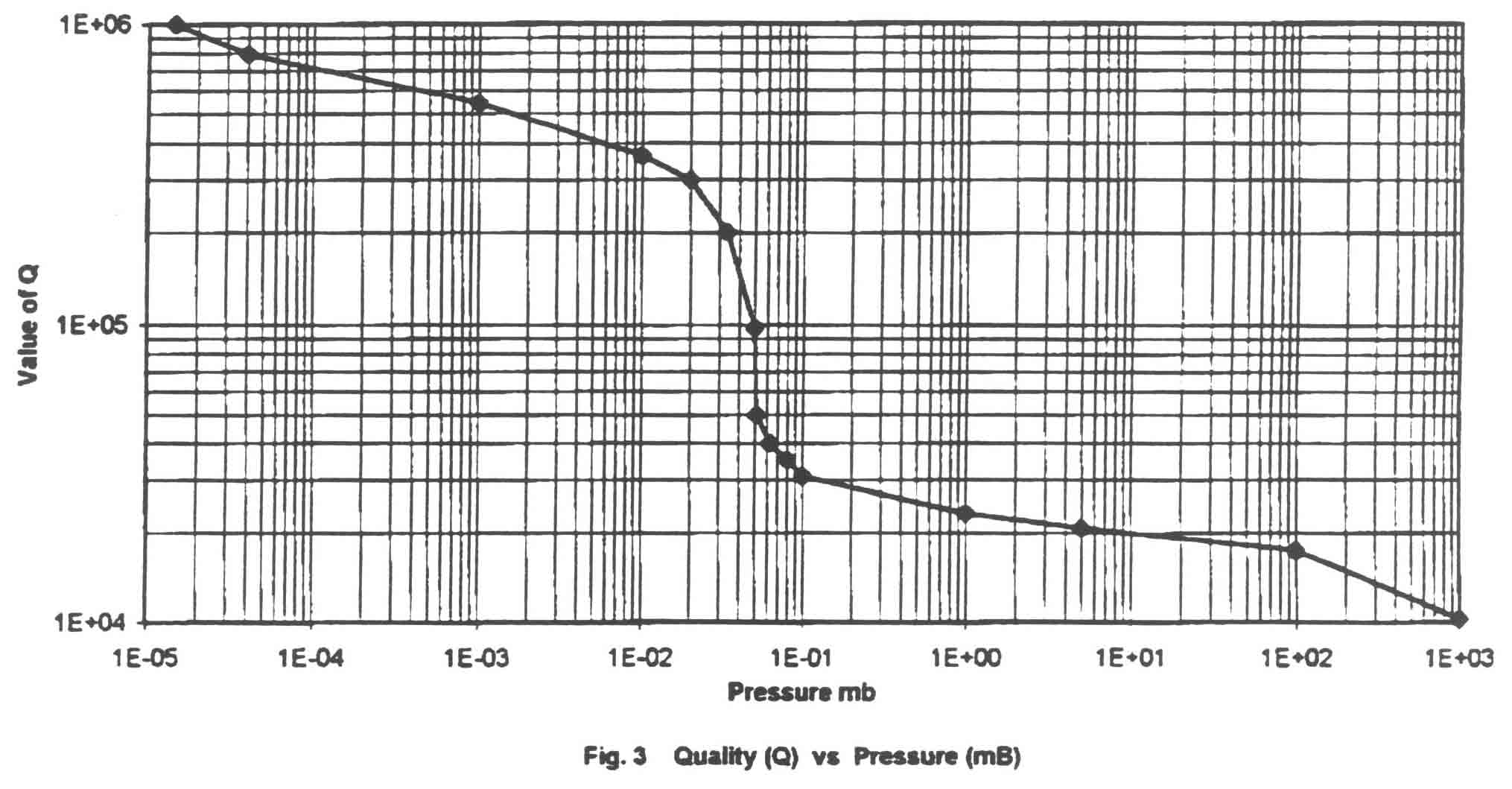
- Calculation of Q.
Q, the 'quality' factor can be calculated from measurements of the time taken for the amplitude
to decay between set values, using the formula:
Q = Π*T/(2*ln(A1/A2)) .............1
Fig. 3 shows the value of Q as plotted against the clock pressure. It will be seen that the value of Q increases comparatively slowly from atmospheric pressure to about 0.1 mb in an inverse fashion.
This range of pressure is in the, so called , "laminar flow" range. Between 0.1 mb and 0.01 mb we move to the "molecular flow" mode and, as can be seen, the value of Q rises much more rapidly with pressure decrease; the value of Q at 2*10-6 mb being about 1,200,000.
The drag coefficient (CD) of a cylindrical pendulum is a function of the Reynolds number (R) only and this will vary with the gas pressure and in particular as to which regime (laminar, low R or turbulent, high R) is prevalent.1 The science of Reynolds numbers is complex, but, as far as we are concerned, it is only the principle which matters; actual calculations are not provided here.
- Calculation of energy requirements.
Let us assume that we start the pendulum swinging at the set amplitude where the amplitude monitor gives a reading of 3150. We know (see above) that this is equivalent to a half swing of 15 * 4820/3150 = 22.9' i.e. 6.66 * 10-3 rad. (φ 1)
We allow the pendulum to swing until the amplitude is half (ie A2 = 6300) , when the swing will be 3.33 * 10-3 rad. ( φ 2 )
The time for this to occur is T seconds.
If m = the effective mass of the pendulum (6360 gm in our clock)
L = the length of the pendulum (106 cm in our clock )
then the maximum vertical movement (h) = L(1 - Cos φ )
when φ is small, COS φ = 1 - (φ 2/2), so h=L(φ 2/2)
If h1 and h2 are the two vertical heights (at A1 & A2),
Δ h=h1 - h2 = L/2(φ 12 φ 22)
Loss of potential energy during the above experiment (LPE) = m * Δh gm cm
LPE per sec = m * Δh/T gm cm per sec
1 gm cm = 9.807 * 10-5 watts
Watts consumed by clock movement = m * Δh * 9.807 * 10-5 / T watts
or m * Δh * 9.807 * 102 / T ergs per sec
For example by experiment we find the following:
| Pressure (Mb) | Time ( sec) | Q | LPE | Watts | Ergs/sec |
| 1000 | 4545 | 10300 | 11.13 | 2.4 * 10-7 | 2.4 |
| 1 * 10-5 | 530000 | 1.2 * 106 | 11.13 | 2.1 * 10-9 | 2.1 * 10-2 |
It is noteworthy that the energy expended at 1000 Mb is about the same as that expended by a Shortt clock at 3 mb pressure.2 Moreover at very low pressures 100 times less energy is needed as at atmospheric. I believe the agate suspension as opposed to a leaf spring has much to do with these facts.
Calculation of approximate pulse width.
Potential energy at top of swing = Kinetic energy at centre of swing
If V = velocity of pendulum at centre of swing and g = gravitational constant
mgh = m/2 * V2 or gh = V2/2
From above h = L* φ2/2 or, in our case, h = 0.0023 cm
and V = 2.12 cm/sec
Since the slit width is 1.6 mm, the pulse width should be 0.16 / 2.12 secs or 75 ms: this is in reasonable agreement with that measured below.
- Amplitude 'lock' facility and impulse current.
Despite careful electronic and mechanical design, it has been found that the amplitude sometimes
wanders. This is particularly the case when the suspension is given a jolt (wind?) and it may take
several hours for the amplitude to again stabilise to the original value. To improve this situation
the computer monitors the amplitude value and decides when to provide impulses. At present the
amplitude value 'aimed for' is 3150. If the monitored reading falls below this value no impulse is sent to the impulse coil for a pre set number of seconds ( usually set at 60 sec ).
The current through the impulse coil can be set by potentiometer.
The values, found by experiment at a pressure of 10-5 mb, are approximately:
- Impulse coil resistance = 910 ohms
- Pulse current peak value = 900 μa
- Pulse width = 70 ms
- Repetition rate ( averaged over 1 hr) = 0.25 Hz
- Calibration of pendulum tilt detector.
Let us assume
- Half angle of swing = θ degrees
- Experimental reading = R
- Angular misalignment of pillar = φ degrees
- Linear misalignment of pillar over pendulum length = L mm
- Then φ= R * θ / 2* 500000
- If 0 = 0.25 and R = 1, then φ = 2.5 * 10-7 degrees or approx. 10-3 arc seconds
- If the pendulum length (between suspension and slot) = 1120 mm
- then L = 1120 * Tan φ
- or using the above conditions, L = 5 * 10-6 mm = 5 * 10-3 μ M
In practice it has been found, over a long period, that the recorder shows a maximum deflection of about ± 10 mm, representing some ± 0.25 arc seconds of tilt.
- RESULTS
- Amplitude stability.
Constant amplitude is entirely dependant on the stability of the suspension. It would appear that
such possible variations as impulse current drift, temperature changes, pressure variations or
changes of current in the coaxial bias coil are either too small to have an effect or are suitably compensated.
Fig. 4a shows variations of amplitude with a moderate breeze blowing when the clock was suspended from a concrete pillar 35 cm square cross section, the base of the pillar being attached to the 15 cm thick concrete raft of the workshop. It is relevant to mention that a large chestnut tree is only 2 meters from one end of the raft.
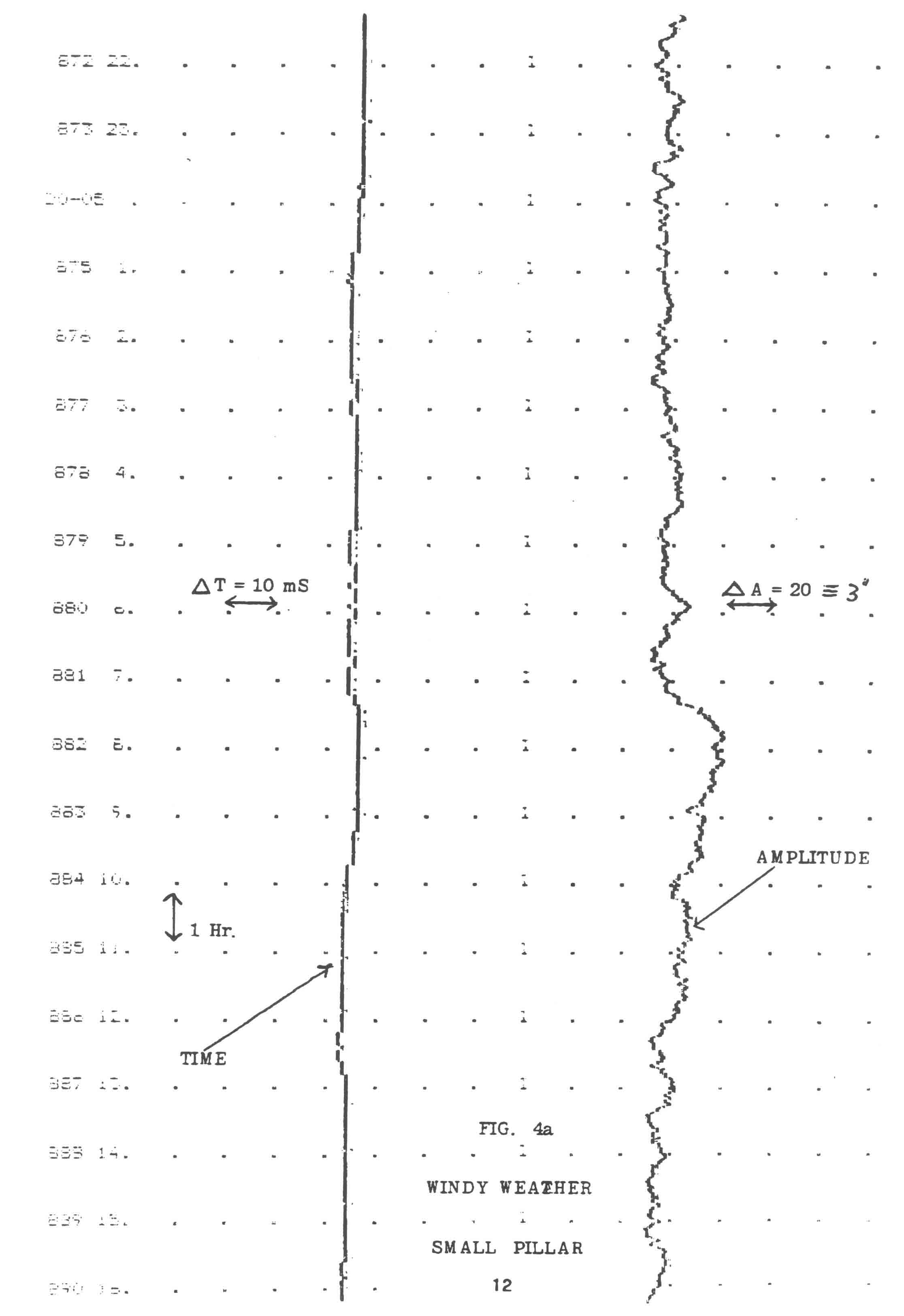
Figure 4a - Windy Weather - Small Pillar
With the clock suspended from a large buried concrete platform measuring 120 x 120 x 300 cm deep below ground and with a pillar 60 x 60 x 250 cm high above ground; the estimated weight of the platform is 12 tonnes. The two portions of the concrete construction were poured at the same time and joined by non magnetic stainless steel tie rods, 25 mm diameter.
Care was taken so that the concrete block was completely mechanically unconnected to the original building; moreover an isolating sleeve of 50 mm thick expanded polystyrene was placed between the underground concrete and the surrounding walls. The concrete was poured onto a consolidated sandy base.
Fig. 4b provides evidence of greatly improved stability when the wind conditions were very stable;. as can be seen the amplitude scarcely changes over many hours.
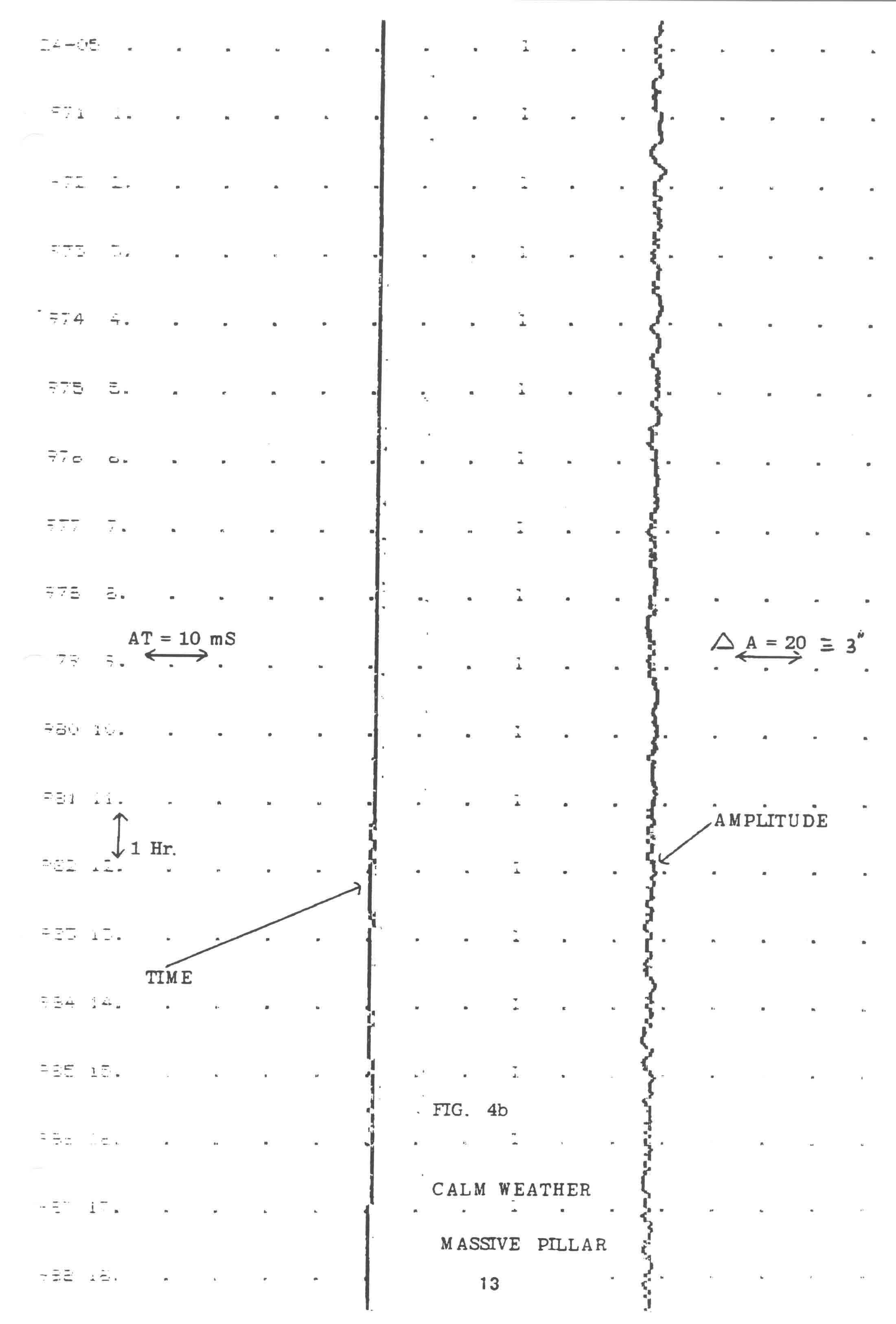
Calm Weather - Massive Pillar
Fig 4a shows a maximum variation of some ± 1.5" in amplitude (calculated from the amplitude readings shown). Reference to Rawlings3 shows that if the amplitude = α° and the variation of amplitude = ±φ minutes of arc, then the circular error will be ± 1.645 ( α°)2 * φ' . This means that in our case the circular error will not exceed 0.2 ms/Hr.
However since amplitude changes will be plus and minus, the average figure will be much less. Indeed the computer shows that the average hourly amplitude does not change by more than ± 2 units, showing a rate change of some 1ms/day as a more likely figure.
- Time stability.
Fig. 5a and 5b demonstrate typical variations of time change over a few hours. The improvement
in performance with wind conditions will be seen.
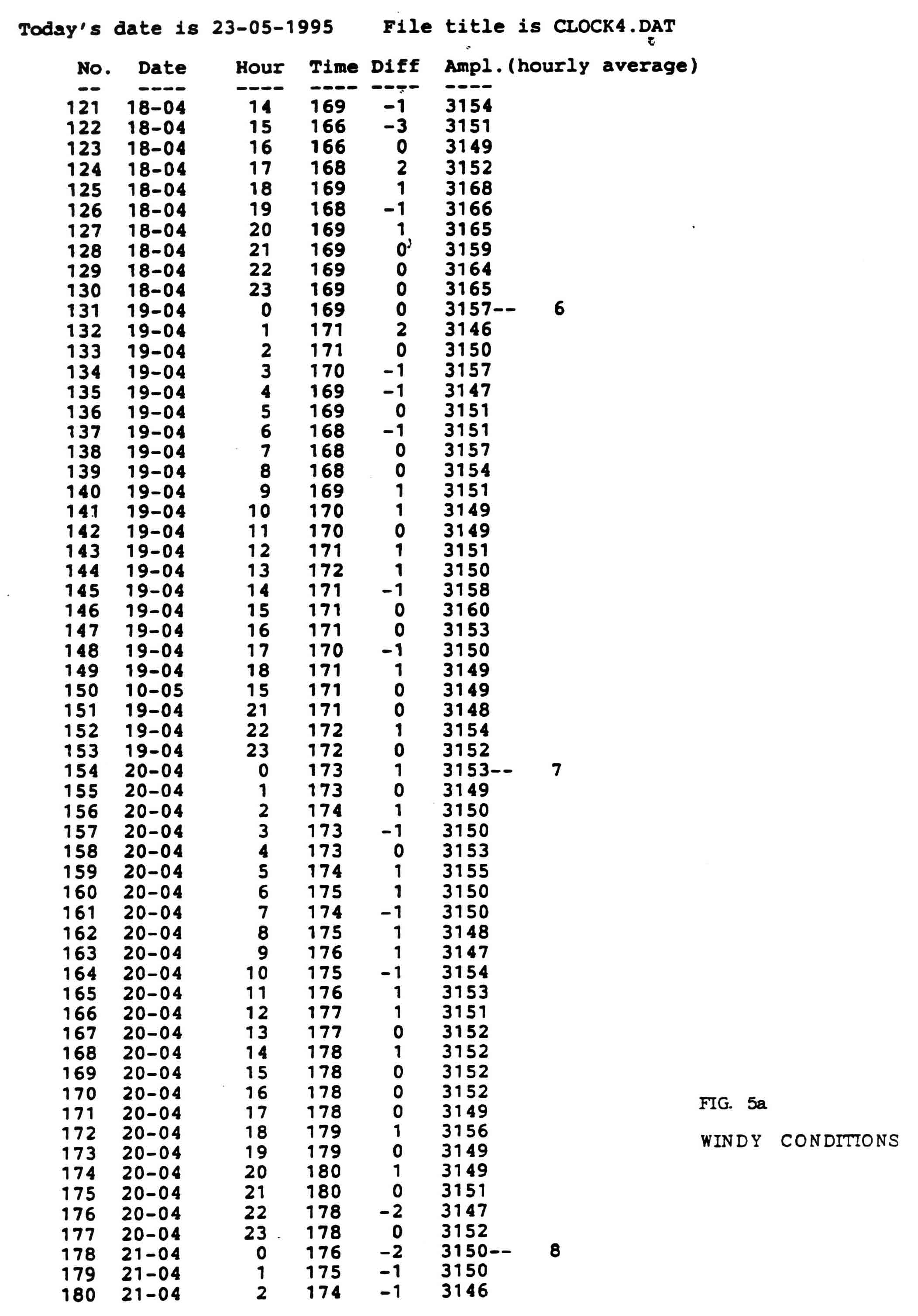
Figure 5a - Windy Co0nditions
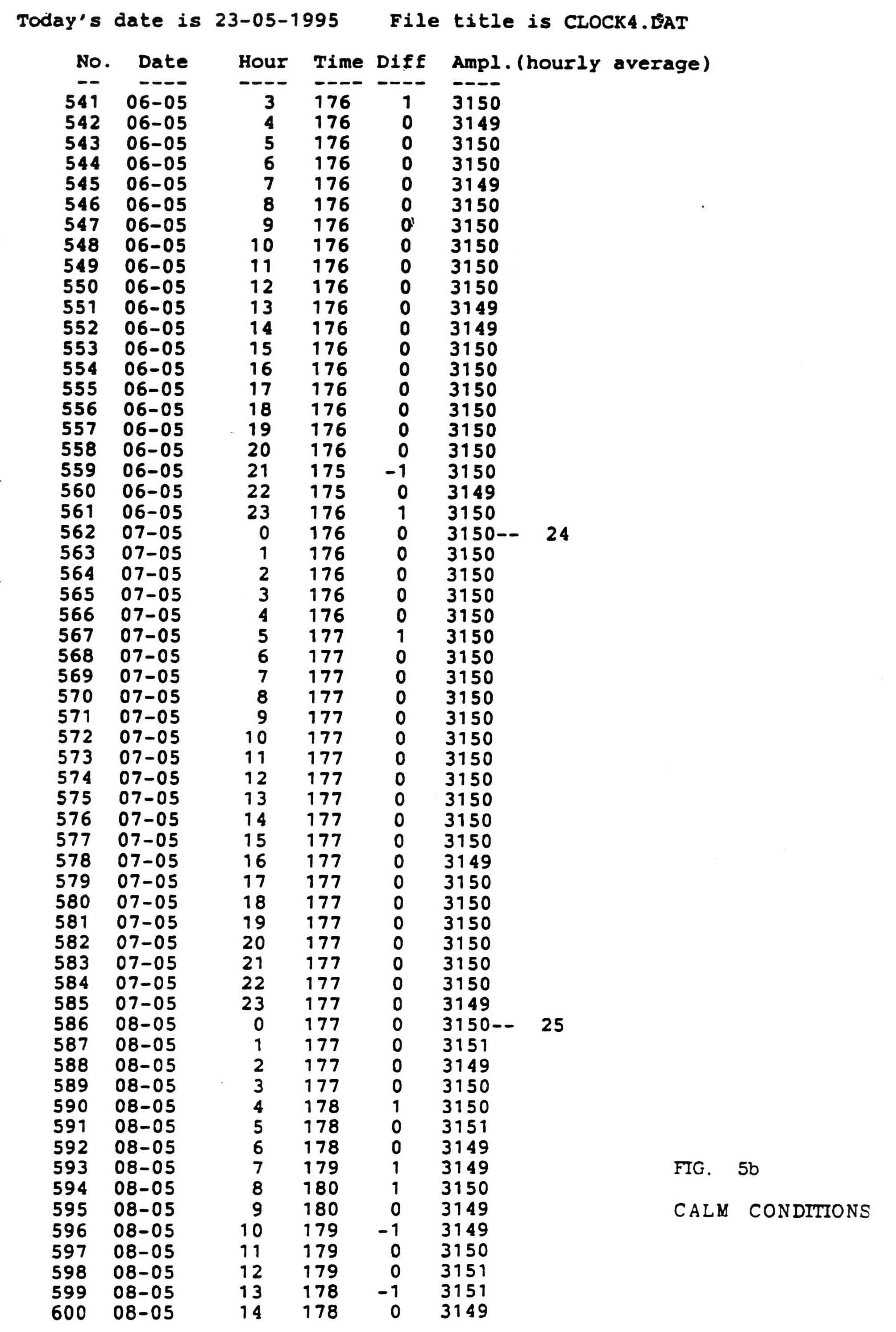
Figure 5b - Calm Conditions
The bias current (see Adjustment of Rate method 3 above) is very carefully adjusted to give zero
drift over many days; after 50 days, the variations from mean time amount to some ± 10 ms.
Fig. 8 shows a smoothed (averaged over 48 hour periods). It can be seen that, over a 250 day
period the median time value has varied by some ± 30 ms based on these 48 hour averages.
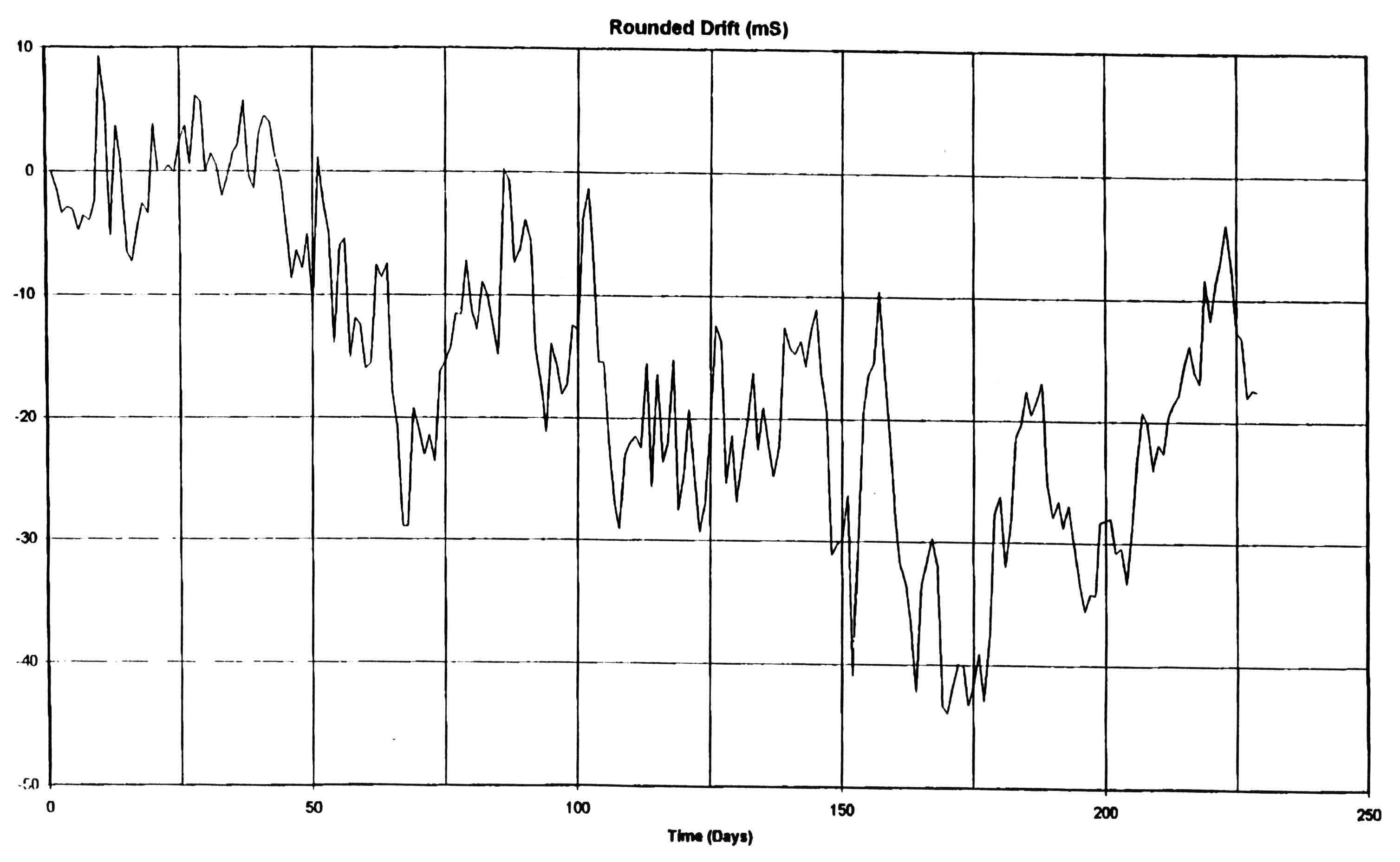
Figure 8 - Drift
- Allan variation.4
This method of estimating the stability of clocks was devised by David Allan of the US National
Bureau of Standards and is a particular method of applying a "root mean square" analysis of the
differences of rate recorded (in my case) every hour. The reader should read the reference given.
The curve produced is the ultimate test of performance. Fig. 6 gives a list of values of Allan
variation and of fractional frequency fluctuation (ΔF/F). These measurements have been
progressing for some 8 months (as at 1/6/96). More time is required for a final comparison with
other clocks.
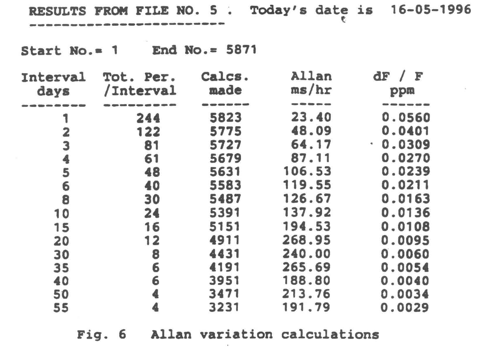
We can calculate the gradient of the Allan curve as follows:
- If, from Fig. 6, the interval and dF/F at any particular time are I1 and F1 etc.,
the Allan gradient will be (log F2 - log F1) / (log H2 - log H1)
- Using this formula with the figures in Fig. 6, we find that the gradient is -0.5 ± 0.05
- This result is described as "ideal" in Ref.4 p.364.
- Comments.
- The accuracy of our clock is largely dependent on the rigidity of the suspension.
- The shape of my Allan curve (see Fig. 7) is approximately what one would expect, if little drift
was being experienced . In Fig. 7b my results are added to those plotted by Philip Woodward
showing the curves obtained from various other clocks. The contrasts are noteworthy 5
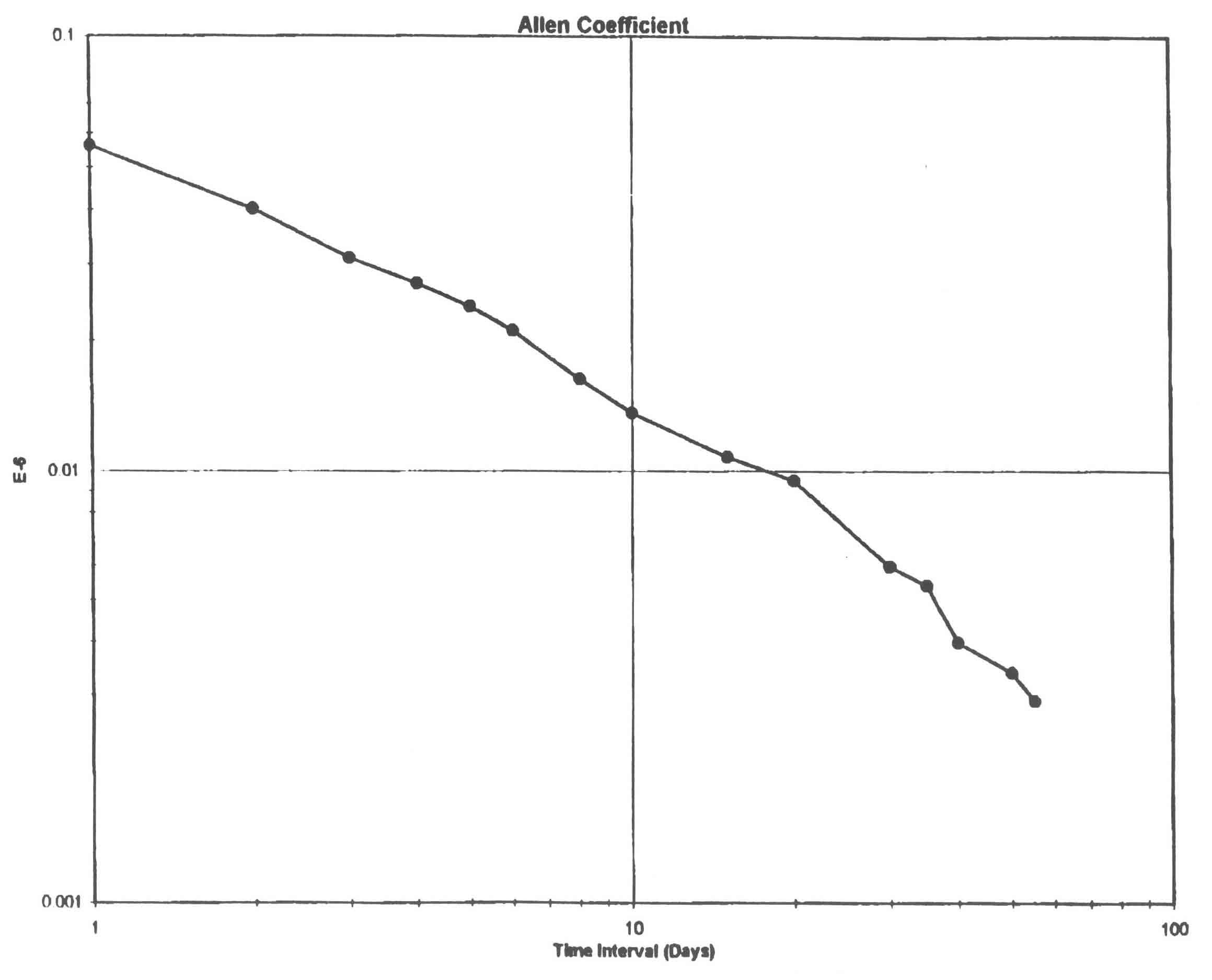
Figure 7
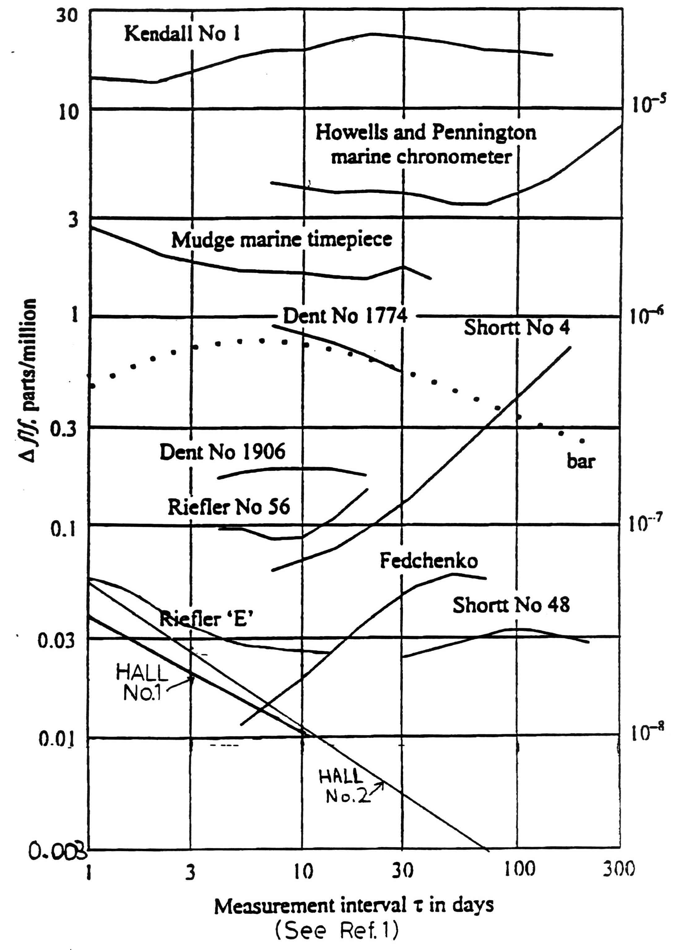
Figure 7b
- The Invar pendulum was thought to be stable after some 15 years after manufacture. However
during the last few months some evidence of "growing" looks possible.
- The Allan Coeficient after some 8 months is approx. 3*10^ 9.
- The Future. In the next few weeks I intend to eliminate any possibility of pendulum creep by changing the material used to a glass/ceramic; either Zerodur (Schott of Germany) or ULE (Corning). If I can afford it ! If I can't, I'll use quartz.
1. American Inst. Phy. Handbk. 3rd Ed. McGraw Hill Bk. Co., p. 2 266.
2. Rawlings, A L , The Science of Clocks & Watches, 3rd Edition 1993, p.55
3. Ibid. p. 360
4. Ibid. p. 153
5. Ibid. Chap. 18 by Philip Woodward. D.Sc.